Drawing perfect spheres, cylinders, and capsules in only 2 triangles.

An efficient 3D molecular rendering method.

>

---

To visualise atoms an molecules often you want to draw spheres and cylinders. Spheres for the atoms (sometimes scaled to their Van der Waals radius, an equilibrium point [1]) and cylinders for the bonds. The classic ball and stick approach. The problem is that spherical objects, at first glance, require an infinite number of triangles to render smoothly with a mesh. There are multiple procedural mesh refinement methods that can do this to any degree. But the cost is a large number of triangles. Possibly 100,000s for a visually pleasing sphere. If we want to render 1,000,000s of atoms this is not going to work. There is a solution though - ray-tracing in the fragment shader.

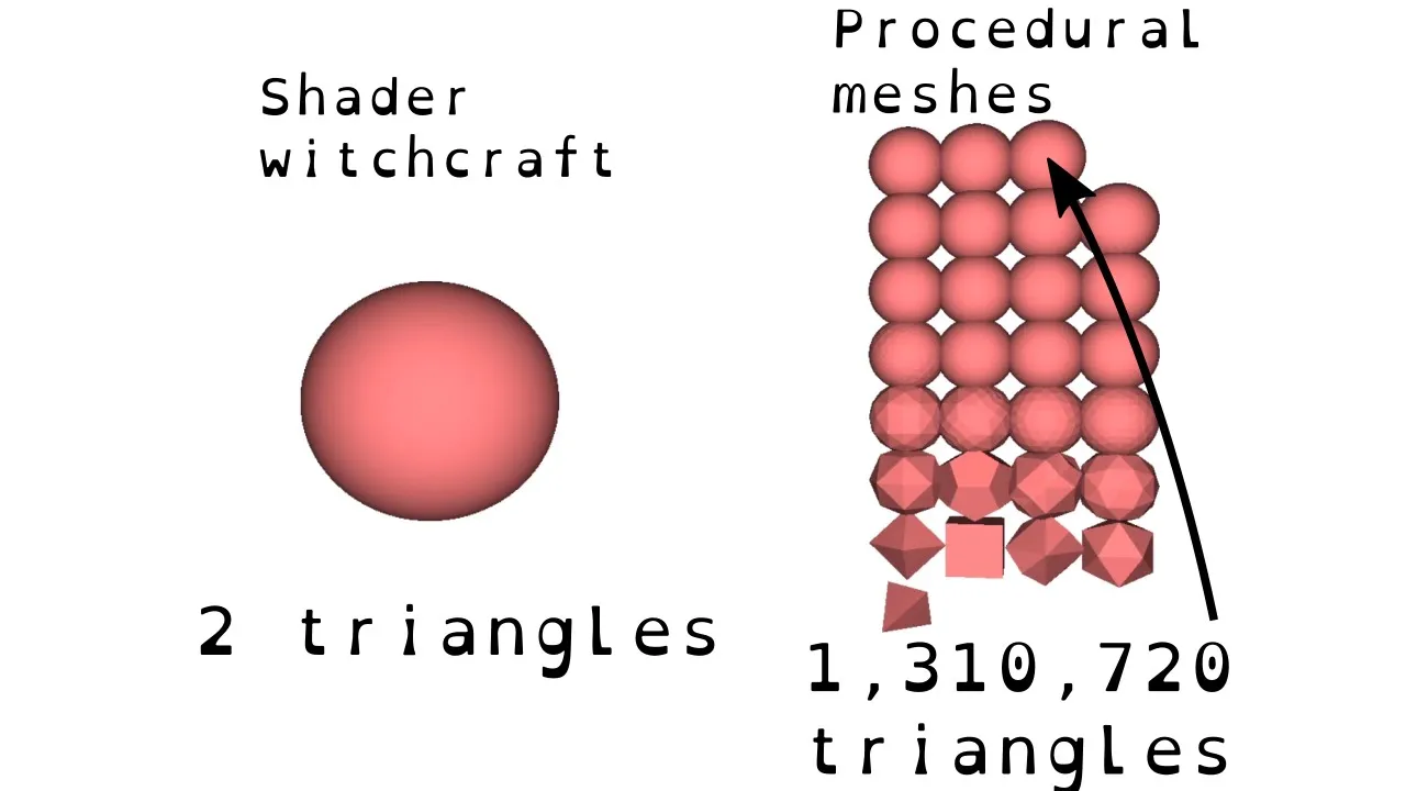
Ray-tracing is in general also quite a brutal performance cost. But to render a sphere we don't need Physically Based Rendering (PBR): materials, reflection, refraction, rays bouncing between objects etc. We just need rays to hit or not hit objects taken one at a time. This boils down to the distance between a line and a sphere (with the right setup).

The general way this is achieved is to

1. Render a quad for the sphere that always faces the camera (billboarding).
2. Operate in view space (so the rays come from \(0,0,0\)).
3. Use fragments on the quad to test for intersection with the sphere.
4. Manipulate gl_FragDepth for correct 3D depth.
5. Instance render for many spheres.

A good tutorial for those nuts and bolts for spheres is online by Jason L. McKesson [2]. The intersection tests (and then normal vector calculations) are simple for a sphere. The two finicky details are (i) the direct manipulation of gl_FragDepth which accounts for the fact we are really rendering a quad in 3D which has a set depth, but want to fake a 3D sphere which clearly has different depth values, and (ii) scaling up the quad to avoid clipping the projected sphere. Both described in [2].

We are going to ray-trace cylinders and capsules as well (cylinders with spheres on the ends). But the methodology is the same. Just different hit geometry. We'll start by setting up the ray-tracing problem as usual in view space. [Warning this is where the algebra starts!]

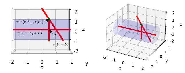
In view space a ray is pointing in \(\boldsymbol{r}(t) = t\hat{{\bf v}}\). Define a line segment starting at \(\boldsymbol{a}\) and ending at \(\boldsymbol{b}\). Finally define a line \(\boldsymbol{l}(s) = \boldsymbol{a}+s\hat{\boldsymbol{n}}\), and a radius \(R\). Let's collect some fun geometry facts:

• The distance between our ray and our line is \(d_{rl}(t) = ||\boldsymbol{a}-\boldsymbol{r}(t)-[(\boldsymbol{a}-\boldsymbol{r}(t))\cdot\hat{\boldsymbol{n}}]\hat{\boldsymbol{n}}||\) [3].
• The ray hits the surface of an infinitely long cylinder defined by this line and radius if and only if \(d_{rl}(t) = R\). There will be two such points (unless we are inside looking directly down the midline), one near and far. Call the one closest to the camera \(\boldsymbol{h}=t^*\hat{\boldsymbol{v}}\).
• The normal vector at the hit point for the infinite cylinder is the unit vector from the point \(\boldsymbol{m}\) along the midline at distance \(R\) to the hit point, back to the hit point.
• \(d_{rl}(t^*)=R\) gives us \(\boldsymbol{m}=\boldsymbol{a}-\boldsymbol{r}(t^*)-[(\boldsymbol{a}-\boldsymbol{r}(t^*))\cdot\hat{\boldsymbol{n}}]\hat{\boldsymbol{n}}\).
• The distance along the midline from \(\boldsymbol{a}\) is \(s=(\boldsymbol{a}-\boldsymbol{r}(t^*))\cdot\hat{\boldsymbol{n}}\)
• The hit point is on the finite capsule if \(s\in [-R, ||\boldsymbol{b}-\boldsymbol{a}||+R]\), and on a finite cylinder if \(s\in [0, ||\boldsymbol{b}-\boldsymbol{a}||]\).
• The normal vector, for a cylinder, is \(\frac{\boldsymbol{a}-\boldsymbol{b}}{||\boldsymbol{a}-\boldsymbol{b}||}\) if \(t = 0\), \(\frac{\boldsymbol{b}-\boldsymbol{a}}{||\boldsymbol{a}-\boldsymbol{b}||}\) if \(t = ||\boldsymbol{b}-\boldsymbol{a}||\), and \(\hat{\boldsymbol{n}}_{cap}=\frac{\boldsymbol{h}-\boldsymbol{m}}{||\boldsymbol{h}-\boldsymbol{m}||}\) otherwise.

What we have is a single equation. This distance will involve a square root, so we actually solve for \(d_{rl}^{2}(t) = R^2\). Which gives us a quadratic in \(t\). Looking at the figure this makes sense given the ray will pass throught the cylinder. The smallest solutuion will be the hit point closest to the camera.
Muscling throught it we get,

$$ \begin{aligned}d_{rl}^{2}(t) &= (\boldsymbol{a}-\boldsymbol{r}(t)-[(\boldsymbol{a}-\boldsymbol{r}(t))\cdot\hat{\boldsymbol{n}}]\hat{\boldsymbol{n}})\cdot(\boldsymbol{a}-\boldsymbol{r}(t)-[(\boldsymbol{a}-\boldsymbol{r}(t))\cdot\hat{\boldsymbol{n}}]\hat{\boldsymbol{n}})\\&=(\boldsymbol{a}-\boldsymbol{r}(t))\cdot(\boldsymbol{a}-\boldsymbol{r}(t))+[(\boldsymbol{a}-\boldsymbol{r}(t))\cdot\hat{\boldsymbol{n}}]^{2}-2(\boldsymbol{a}-\boldsymbol{r}(t))\cdot[(\boldsymbol{a}-\boldsymbol{r}(t))\cdot\hat{\boldsymbol{n}}]\hat{\boldsymbol{n}}\\&=\boldsymbol{a}\cdot\boldsymbol{a}+\boldsymbol{r}(t)\cdot\boldsymbol{r}(t)-2\boldsymbol{a}\cdot\boldsymbol{r}(t)+[(\boldsymbol{a}-\boldsymbol{r}(t))\cdot\hat{\boldsymbol{n}}]^{2}-2(\boldsymbol{a}-\boldsymbol{r}(t))\cdot[(\boldsymbol{a}-\boldsymbol{r}(t))\cdot\hat{\boldsymbol{n}}]\hat{\boldsymbol{n}}.\end{aligned}$$ Now, $$\begin{aligned}((\boldsymbol{a}-\boldsymbol{r}(t))\cdot\hat{\boldsymbol{n}})^{2} = (\boldsymbol{a}\cdot\hat{\boldsymbol{n}})^{2}+(\boldsymbol{r}(t)\cdot\hat{\boldsymbol{n}})^{2}-2(\boldsymbol{a}\cdot\hat{\boldsymbol{n}})(\boldsymbol{r}(t)\cdot\hat{\boldsymbol{n}})\end{aligned},$$ and $$\begin{aligned}2(\boldsymbol{a}-\boldsymbol{r}(t))\cdot[(\boldsymbol{a}-\boldsymbol{r}(t))\cdot\hat{\boldsymbol{n}}]\hat{\boldsymbol{n}}\end{aligned} = 2[(\boldsymbol{a}\cdot\hat{\boldsymbol{n}})^2+(\boldsymbol{r}(t)\cdot\hat{\boldsymbol{n}})^2-2(\boldsymbol{a}\cdot\hat{\boldsymbol{n}})(\boldsymbol{r}(t)\cdot\hat{\boldsymbol{n}})].$$ Combining these last two equations we can collect some terms $$d^2_{rl}(t) = ||\boldsymbol{a}||^2+||\boldsymbol{r}(t)||^2-2\boldsymbol{a}\cdot\boldsymbol{r}(t)-(\boldsymbol{a}\cdot\hat{\boldsymbol{n}})^2-(\boldsymbol{r}(t)\cdot\hat{\boldsymbol{n}})^2+2(\boldsymbol{a}\cdot\hat{\boldsymbol{n}})(\boldsymbol{r}(t)\cdot\hat{\boldsymbol{n}}).$$ Setting to \(R^2\) and we have our quadratic $$ t^2(1-(\hat{\boldsymbol{v}}\cdot\hat{\boldsymbol{n}})^2) + 2t[(\boldsymbol{a}\cdot\hat{\boldsymbol{n}})(\hat{\boldsymbol{v}}\cdot\hat{\boldsymbol{n}})-\boldsymbol{a}\cdot\hat{\boldsymbol{v}}]+||\boldsymbol{a}||^2-(\boldsymbol{a}\cdot\hat{\boldsymbol{n}})^2-R^2 = 0.$$ Defining \(\alpha=\boldsymbol{a}\cdot\hat{\boldsymbol{n}}\), \(\beta=\hat{\boldsymbol{v}}\cdot\hat{\boldsymbol{n}}\), and \(\delta=\boldsymbol{a}\cdot\hat{\boldsymbol{v}}\). The roots are $$t_{\pm} = \frac{-(\alpha\beta-\delta)\pm\sqrt{(\alpha\beta-\delta)^2-(1-\beta^2)(||\boldsymbol{a}||^2-\alpha^2-R^2)}}{(1-\beta^2)}. $$ Which is a little hairy... but we have our solutions \(t_{\pm}\hat{\boldsymbol{v}}\) from which we take the smallest as our \(t^*=\text{min}(t_{+},t_{-})\).
Using this we have our mid point and normal vector $$ \begin{align}\boldsymbol{m}&=\boldsymbol{a}-\hat{\boldsymbol{v}}t^*-[(\boldsymbol{a}-\hat{\boldsymbol{v}}t^*)\cdot\hat{\boldsymbol{n}}]\hat{\boldsymbol{n}},\\\hat{\boldsymbol{n}}_{cap}&=\frac{[(\boldsymbol{a}-\hat{\boldsymbol{v}}t^*)\cdot\hat{\boldsymbol{n}}]\hat{\boldsymbol{n}}-\boldsymbol{a}}{R}\end{align}, $$ and using the same OpenGL incantations as [2] (but with instanced rendering) that's a wrap!

Don't forget to checkout the code on Github https://github.com/JerboaBurrow/SimpleFastOpenAtomicVisualiser

---

---